
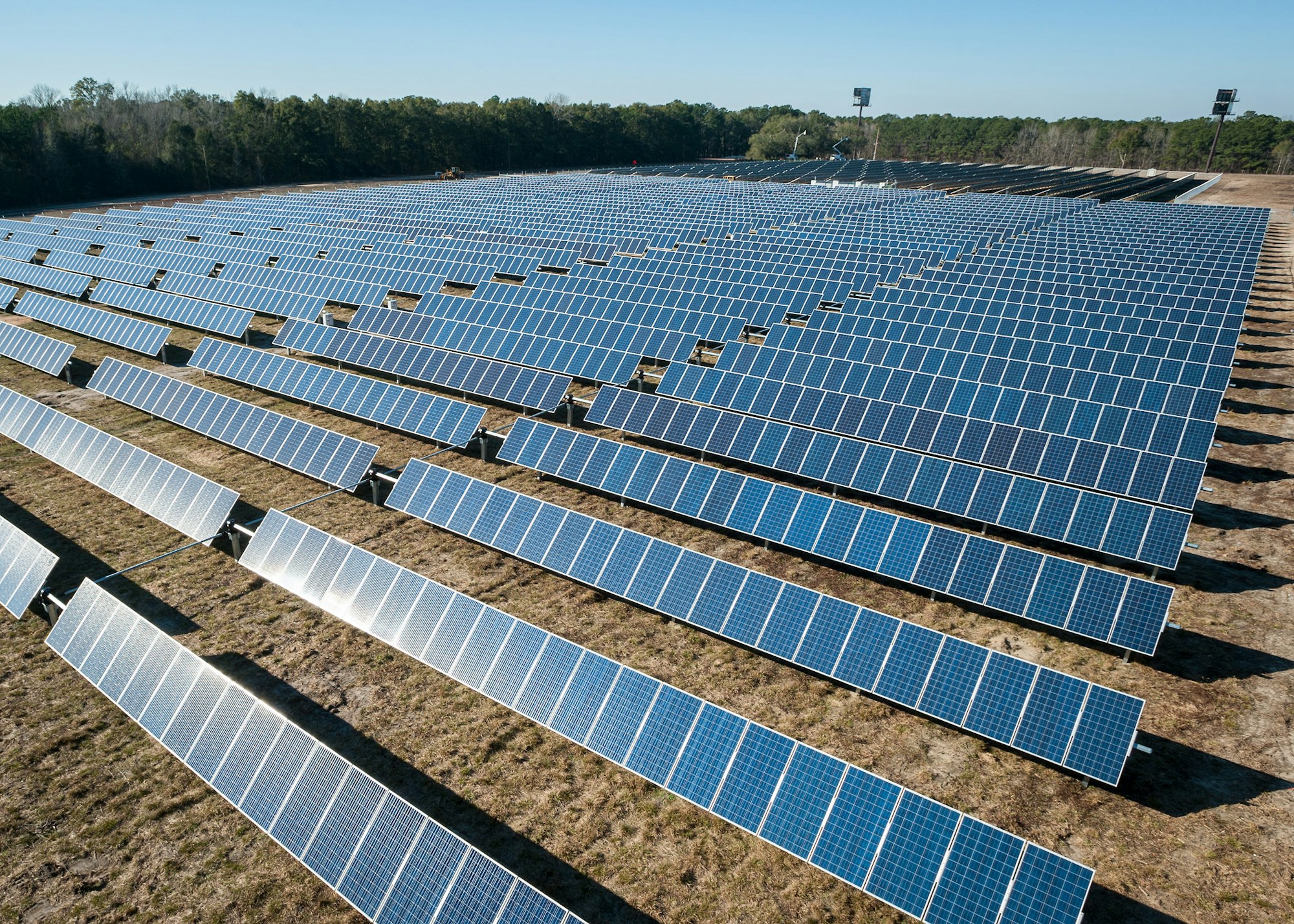
As hardware costs continue to decline, designers are squeezing more solar modules into each system. By shrinking the spacing between the rows of modules, they get larger systems – maximizing overall energy production, and improving the cost-benefit of the array.
However, the tighter spacing has very different effects depending on whether the array uses fixed-tilt racking, or a tracker system. And ultimately, we find that the tracker systems’ performance advantage versus fixed-tilt systems shrinks in this new design paradigm.
As a result, the rules of thumb for tracker performance advantages that were appropriate 5-10 years ago are becoming outdated today. Specifically, the “15 to 20% energy yield improvement” may no longer be true.
The Comparison
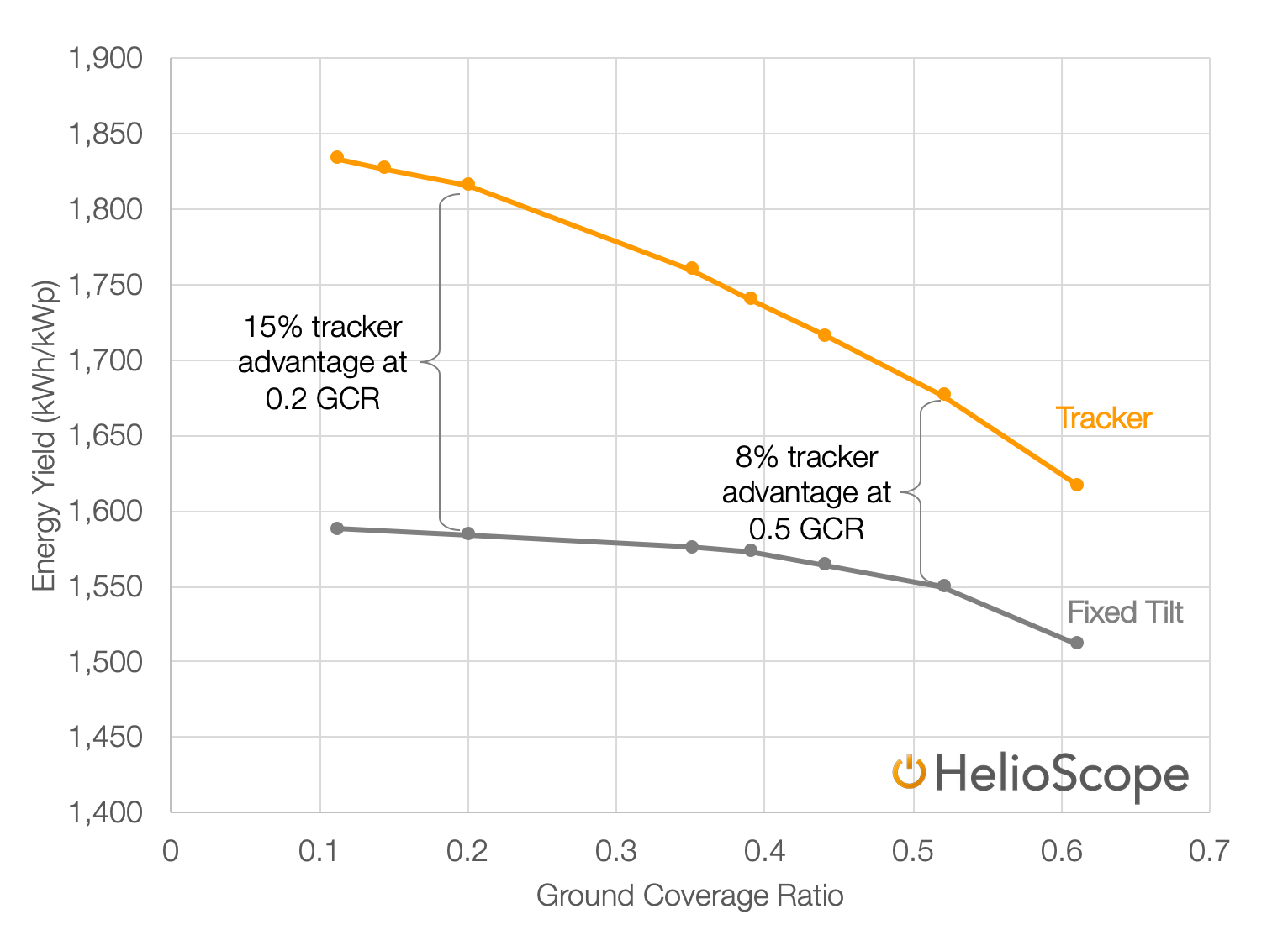
Let’s first look at the fixed-versus-tracker comparison in the ‘old’ paradigm of wide spacing between rows. In Charlotte, comparing a fixed-tilt system to a tracker at a 24’ row spacing (representing a 0.2 ground coverage ratio, or “GCR”), the tracker improves yield approximately 15%, from 1,585 kWh/kWp to 1,815 kWh/kWp. In a sunnier Phoenix with the same designs, the tracker benefit is even higher, with a 20% performance advantage over fixed-tilt.
However, if we switch to closer spacing (spacing of approximately 6’, equivalent to a 0.5 ground coverage ratio), the tracker benefits compared to fixed-tilt become slimmer. All of the numbers fall, of course, as squeezing the modules closer together will naturally reduce the energy yield per watt of capacity. But the fixed-tilt systems fall only modestly (about 2% in both Charlotte and Phoenix), while the tracker yields fall more significantly, by 8-9%. As a result, the tracker yield advantage over fixed-tilt falls to about 8% in Charlotte and about 12% in Phoenix – in both cases, losing nearly half of the advantage.
The Anatomy of Tighter Spacing
To understand why the two systems respond so differently, we look deeper at the performance calculations.
For the fixed-tilt scenarios, the main parameter that changes is the shading loss. This makes sense: as the modules are closer together, they shade each other more:
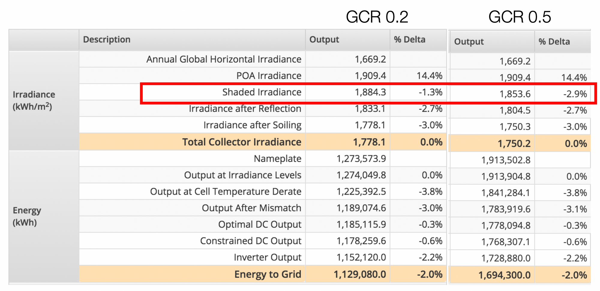
However, when we run the same analysis on a tracker system, we see very different behavior:
While the fixed-tilt arrays saw shading losses for the tightly-packed systems, the tracker system’s production decrease is mostly caused by POA losses – a difference of over 5% between the two cases.
Why Does Plane-of-Array Change? Backtracking.
The Plane-of-array (POA) calculation in solar modeling shows how much additional sunlight the modules get because of their tilt, compared to a flat module on the ground. This value can be zero (for a module with a tilt of 0°), is typically +3% to +15% for a fixed-tilt array (depending on the tilt) and can be upwards of +20% to +30% for a single-axis tracker array (since, in that case, the plane of the array actually tracks with the sun throughout the day). (The Plane of Array calculation can even be negative, if the array is pointed away from the equator.)
The main reason for the drop in POA is the fact that tracker systems will backtrack to avoid row-to-row shading.
Coming back to the tracker production: the main reason for the drop in POA is the fact that tracker systems will backtrack to avoid row-to-row shading. At the beginning and end of the day, the tracker system will reverse the modules’ tracking in order to prevent them from shading each other. As a result, when the sun is at the horizon, the modules are actually flat (to avoid shading) rather than being tilted up at 90° (to be pointed directly at the horizon).
Note that when a tracker is backtracking, it is actually sacrificing its orientation toward the sun in order to prevent module shading. In general, this produces more energy than tracking the sun and incurring shade (and mismatch) losses.
For arrays with higher GCR values, backtracking happens more often and more significantly. When the tracker rows are spaced more closely together, they end up blocking each other later in the morning and earlier in the evening. A tracker system with a GCR of 50% will end up backtracking for over 1,720 hours over the course of a year, over a third of the operating hours of the array, representing about 25% of the array’s annual energy yield.
In fact, we can actually calculate the tilt angle where backtracking will begin, based on the GCR of the array. For example, at a GCR of 0.4, the trackers can reach a tilt angle of 63° before they have to begin backtracking. But at a tighter GCR of 0.55, the trackers will begin to shade each other (and therefore begin backtracking) at a tilt of just 52°.
Backtracking means that the losses from tighter spacing in tracker systems show up in the “Plane of Array” (POA) step of the calculations. While this may make logical sense, this can lead to confusion: POA is the step where the tracker systems’ boost shows up. Yet with backtracking, this calculation essentially conflates two factors: the boost from trackers, and then the losses from backtracking.
Conclusion
And ultimately, tracker systems still make a ton of sense in a lot of locations, since the cost increase is often smaller than the yield increase. But today’s designers and developers would be wise to confirm their yield expectations based on the system location and design, rather than just based on their rule-of-thumb yield expectations.